Gravity++
A finite-volume moving-mesh code for compressible hydrodynamics and ideal magnetohydrodynamics.
Code Summary
Gravity++ is designed for high-fidelity astrophysical fluid simulations on Voronoi meshes. The solver stack combines Godunov fluxes, second-order MUSCL-Hancock time integration, adaptive moving meshes, and an MHD module with divergence control.
Numerics
Finite-volume Godunov method on 3D Voronoi cells.
Accuracy
Second-order in space and time through MUSCL-Hancock.
Mesh
AREPO-style moving mesh using Voro++ tessellation.
I/O
HDF5 workflow compatible with AREPO-like snapshots.
Ideal MHD Equations (Conservative Form)
Gravity++ uses the standard ideal-MHD system (in code units with mu0 = 1):
For divergence control, Gravity++ supports Dedner cleaning workflows and constrained transport paths.
MUSCL-Hancock: Second-Order in Space and Time
The update is performed through a predictor-corrector sequence designed for robust shock capturing and low diffusion in smooth regions:
- Compute cell gradients with Green-Gauss / least-squares estimators.
- Apply slope limiting (TVD family) to prevent non-physical oscillations.
- Reconstruct left/right primitive states at each face center.
- Predict half-step states using local temporal derivatives.
- Solve face Riemann problems and update conserved variables with face fluxes.
- Advance Voronoi generators and rebuild the tessellation for the next step.
Riemann Solvers: Exact, HLLC, HLLD
| Solver | Primary Use | Wave Model | Notes |
|---|---|---|---|
| Exact (Euler) | Reference and validation runs | Iterative exact 1D Riemann solution | High-fidelity benchmark for hydro flux verification. |
| HLLC | Default hydrodynamic production solver | Three-wave model (SL, S*, SR) | Good balance of accuracy and robustness for Euler flows. |
| HLLD | Default MHD production solver | Seven-wave MHD structure (fast, Alfvén, contact, slow) | Resolves MHD discontinuities with lower diffusion than HLLE-type fluxes. |
Moving Mesh with Voro++
Gravity++ computes Voronoi geometry (cell volumes, face areas, normals, centroids) with Voro++. The mesh motion follows an ALE-style formulation where generators track flow motion while preserving cell quality.
This construction minimizes advection error, improves Galilean behavior, and preserves sharp structures compared with static-grid approaches.
SoA Architecture and GPU-Oriented Optimization
Gravity++ has a defined migration path toward a Structure of Arrays (SoA) data layout for the heavy compute kernels (gradients, reconstruction, and Riemann flux loops). For GPU execution, this is a core optimization step.
- Contiguous per-field arrays improve cache locality and SIMD utilization on CPUs.
- SoA enables coalesced memory transactions on GPU warps.
- Kernel interfaces become cleaner for OpenMP target, CUDA, and multi-GPU decomposition.
- AoS to SoA conversion is used as an incremental strategy to keep I/O compatibility during migration.
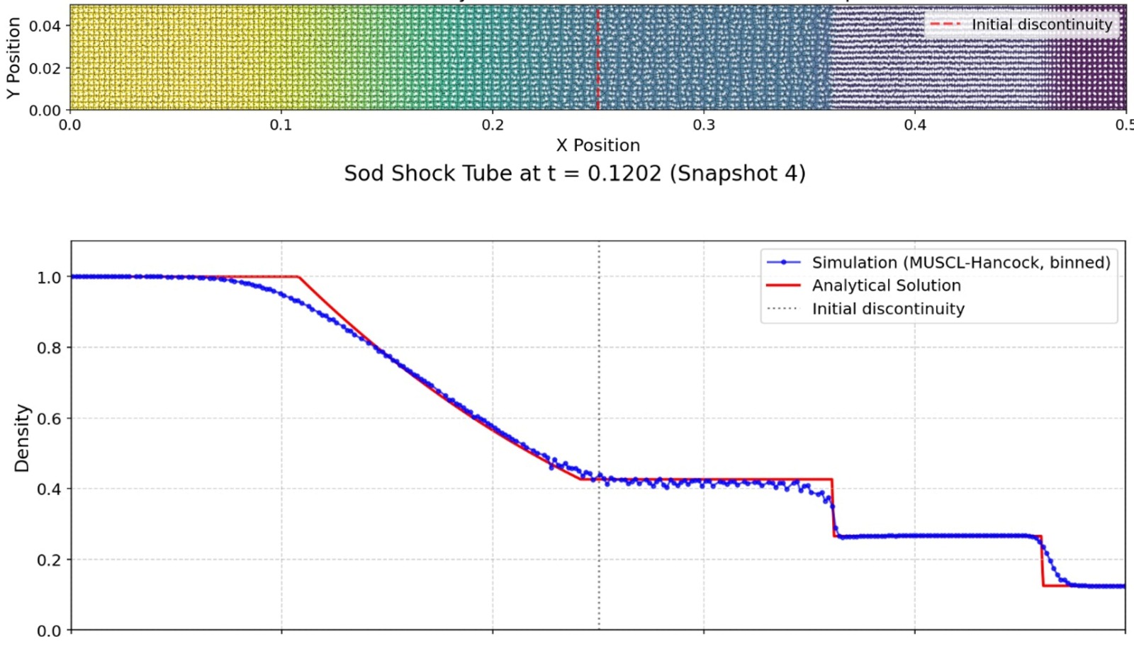
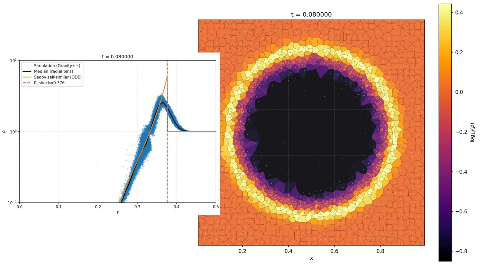
Validation: Sod Shock Tube and Sedov-Taylor Blast
Selected References
- Springel, V. (2010), E pur si muove: moving-mesh hydrodynamics with AREPO, MNRAS 401, 791.
- Toro, E. F. (2009), Riemann Solvers and Numerical Methods for Fluid Dynamics, Springer.
- Miyoshi, T. and Kusano, K. (2005), A multi-state HLL approximate Riemann solver for ideal MHD, JCP 208, 315.
- Dedner, A. et al. (2002), Hyperbolic divergence cleaning for MHD, JCP 175, 645.
- Rycroft, C. H. (2009), Voro++: A three-dimensional Voronoi cell library in C++, Chaos 19, 041111.